

One other important common feature of Econometric models is the concept of Diminishing Marginal Returns to ad spend. This phenomenon describes what happens when you increase ad spend — efficiency goes down. This occurs because you’ve used up all the ‘low hanging’ fruit, and have to expand out to less relevant inventory.
As ad spend increases, all of the most engaged potential users have already been targeted. So as you expand to lower intent audiences, an additional dollar of advertising spend will yield less ROI. This is why you can’t just double your budget on Facebook Ads and expect to get the same return – you’ll almost always see a higher cost per acquisition.
Follow along by making a copy of this model:
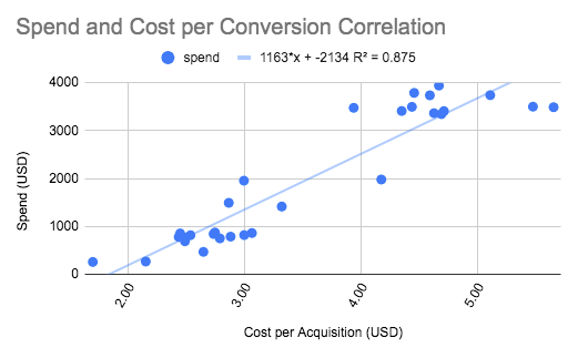
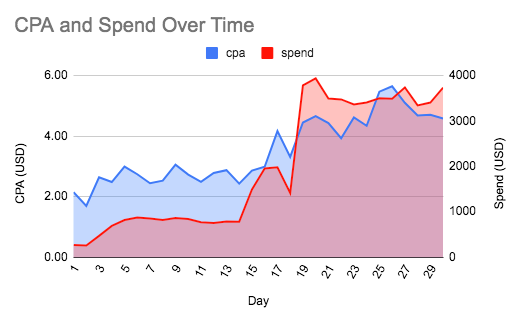
The above is real-world (anonymized) data for a client that increased ad spend from $500 per day to close to $4,000 daily on Facebook ads — they saw their cost per acquisition (CPA) rise 80% from ~$2.50 to $4.50 on average. The coefficient of CPA (x) is telling us that this client will see a $1 rise in cost per acquisition for every additional $1,163 they spend per day.
Seeing diminishing returns as you scale ad spend is fairly typical of the experience of fast-growing advertisers. Until you test and find a winner in terms of ad creative or landing page conversion rate, this pattern will hold. This is precisely why we experiment — it’s only by improving clickthrough rate or conversion rate that we can spend more at the same cost per acquisition (or hold budgets steady and reap the rewards of a lower CPA).
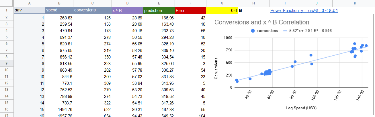
It’s important to note that ad spend doesn’t usually just get less efficient linearly — it often declines at an increasing rate. That means we have to model an exponential decay in our linear regression, which means introducing a non-linear transformation of spend. For this we use the "power function" transformation y=a*x^B. This gives us a nice curve representing the typical effect we expect to see.
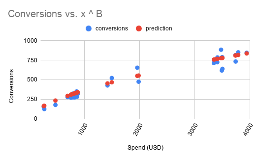
The way we can fit this line in GSheets, is by manually changing the yellow box (B from the equation) until the Prediction values line up with Actuals, the R-squared is at its highest and the Error is at its lowest. Of course professionals would use an automated grid search algorithm for finding what value of B is appropriate, but to keep things simple it’s ok to do this manually.
Now we have a formula that works and is predictive of the relationship between spend and conversions, we can use it to predict CPA at any level of ad spend we like. From the spend and forecast conversions we can work out CPA, as well as the marginal conversions and CPA — i.e. how many extra conversions are we getting from each incremental dollar?
.png)
Now you can see that the increase in CPA was actually worse than you thought — the efficiency of the first $500 or $1,000 was masking the incremental inefficiency of going from say $3,500 to $4,000. From that step change you only get 27 more conversions for your extra 500 dollars, meaning those extra conversions cost you $18.54 each! This effect is called diminishing marginal returns, and it happens whenever you reach saturation in a channel — on the margin conversions get exponentially more expensive.
.png)
It’s important to note that this pattern will be more reliable the closer your historic ad spend has been to the levels you want to experiment with. For example if we’ve never had a $10,000 week, it’s unlikely the model will be very accurate when drawing that curve. I’ve often recommended running a ‘pulse’ test if you need to test a new spend level – arbitrarily spend more some weeks versus others to generate good variance in your data for modeling.
In a real Econometric model you would usually work out the diminishing marginal returns (or efficient frontier curve) for every channel, or even campaign if you had enough data. This would allow you to choose the right budget allocation for each, making tradeoffs between volume and efficiency. This gets at the heart of the strategic value of Econometric modelling – this is how multi-million dollar budgets are confidently justified by the largest advertisers, especially in less directly measurable channels than Facebook ads, like TV, billboards or influencer marketing.
---
That covers how to work Diminishing Returns into your Econometric model, using GSheets. If you haven’t yet read the other posts in this series on Econometrics, you can find the links here:
- Econometrics in GSheets
- Econometrics in Python
- Diminishing Returns (this post)
- Measuring the Halo Effect
- When Econometrics Works
In future we plan to cover:
- Word of Mouth Coefficient
- Testing Model Accuracy
- Monte-Carlo Simulations
- Machine Learning Models
- Data Import from APIs
- The Future of Econometrics
- Any other topics? Tweet @hammer_mt to request

